Advanced probeset selection

In this tutorial we look into customizing the gene set selection for more specific use cases and explore the parameters of the selection procedure.

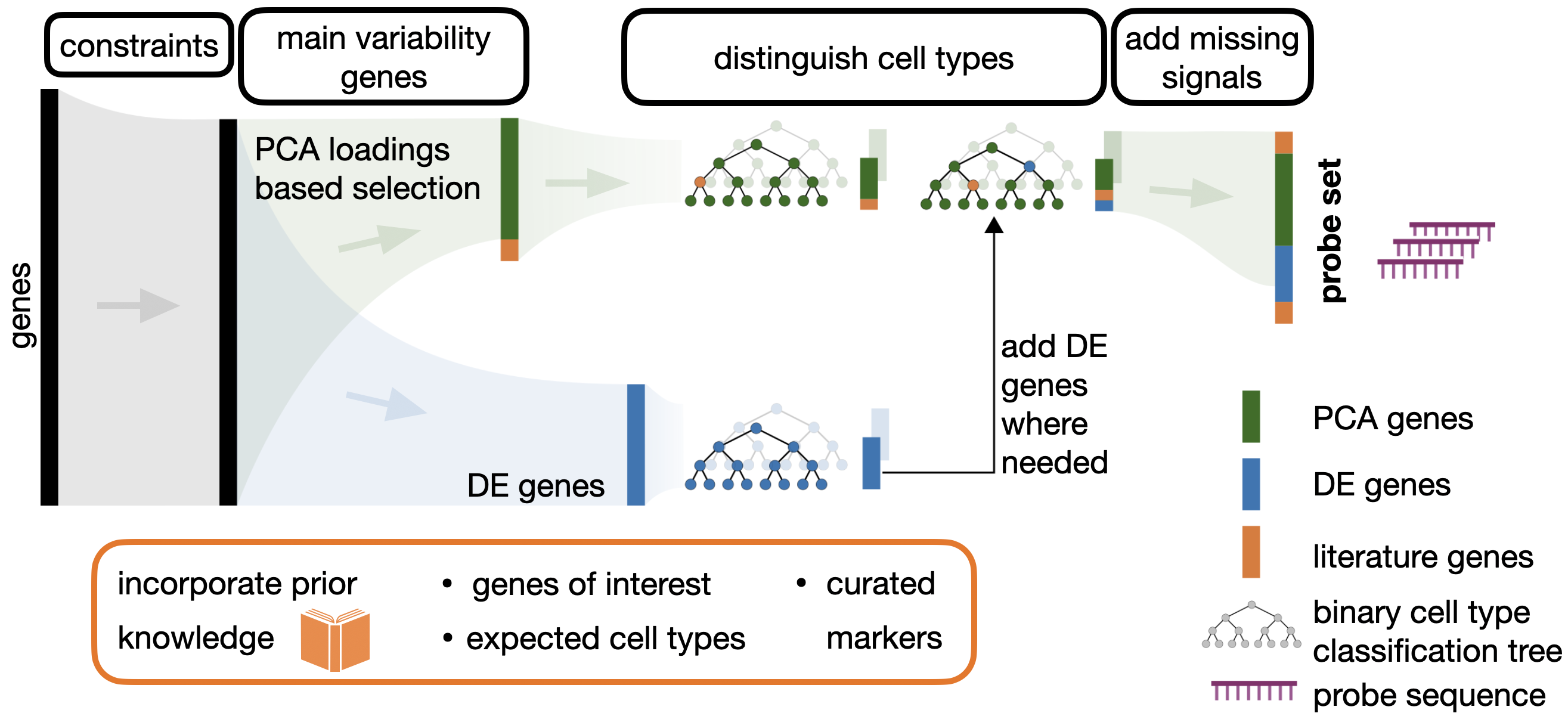
The Spapros probeset selection pipeline simultaneously optimizes for capturing transcriptional variation and cell type identification while taking into account prior knowledge, technical constraints and probe design. The main steps, as visualized in the figure above, are:

Constrains

In the first step, genes are filtered based on technology specific probe design constraints. This part is captured in the end-to-end probeset selection tutorial. (Besides probe design constraints also expression level constraints can be applied as shown in the Selection with experession constraints example below. Those affect multiple steps of the pipeline though)

Variable genes

The next step is a PCA based selection of genes that capture general variation. The subsequent steps of the pipeline are encouraged to select from that set of genes. If you want the selection to be focused only on marker genes and cell type classification, the PCA-based selection step can be omitted, see the Cell type classification only example for this case.

Distinguish celltypes

For each cell type, a binary classification tree is trained on the previously selected gene set. Here the pipeline builds for each cell type a combinatorial rule how to distinguish it from other cell types.

DE gene addition

Similarly to the last step, trees are also trained on DE genes and compared to the trees trained on the PCA based selection. If a DE tree performs better with respect to cell type classification, then DE genes are added to the already selected gene set.

Prior knowledge

There are two possibilities to incorporate prior knowledge. For both, we present use cases in this tutorial:

• Select a few additional genes: pre-selected genes are augmented by combinatorially selecting additional genes around them

• Selection with curated marker list: add markers from a given list in case the signals from that list are not captured with the already selected genes

Probe design

Design the final technology specific probes for the selected genes. As the Constraints step, this part is also only captured in the end-to-end probeset selection tutorial.

Content

0. Import packages

1. Load and preprocess data

2. Use cases

   1. Select a few additional genes

   2. Cell type classification only

   3. Selection for high numbers of genes (> 150)

   4. Selection with curated marker list

   5. Selection with expression constraints

   6. Your use case is not captured?

3. What’s next

0. Import packages

import numpy as np
import scanpy as sc
import spapros as sp

sc.settings.verbosity = 0
sc.logging.print_header()
print(f"spapros=={sp.__version__}")

scanpy==1.9.1 anndata==0.8.0 umap==0.5.3 numpy==1.21.6 scipy==1.7.3 pandas==1.3.5 scikit-learn==1.0.2 statsmodels==0.13.2 python-igraph==0.9.11 pynndescent==0.5.7
spapros==0.1.0

1. Load and preprocess data

For Spapros selections the count data should be log-normalised. Notably genes should not be scaled to mean=0 and std=1. We pre-select a given number of highly variable genes, here 1000. In real world applications we typically go for 8000.

The example data set that we use here has a raw version and a processed version with scaled counts. To get log normalised counts we use the raw version. Cell and gene filters, cell type annotations, and the umap embedding we get from the processed version.

adata = sc.datasets.pbmc3k()
adata_tmp = sc.datasets.pbmc3k_processed()

# Get infos from the processed dataset
adata = adata[adata_tmp.obs_names, adata_tmp.var_names]
adata.obs['celltype'] = adata_tmp.obs['louvain']
adata.obsm['X_umap'] = adata_tmp.obsm['X_umap']
del adata_tmp

# Preprocess counts and get highly variable genes
sc.pp.normalize_total(adata)
sc.pp.log1p(adata)
sc.pp.highly_variable_genes(adata, flavor="cell_ranger", n_top_genes=1000)

adata

AnnData object with n_obs × n_vars = 2638 × 1838
    obs: 'celltype'
    var: 'gene_ids', 'highly_variable', 'means', 'dispersions', 'dispersions_norm'
    uns: 'log1p', 'hvg'
    obsm: 'X_umap'

2. Use cases

We will go through some specific use cases for gene selection.

i. Select a few additional genes

In some situations you already selected multiple genes that you want to measure in a targeted spatial transcriptomics experiment but you still have capacity for further genes. For this scenario the preselected_genes parameter was introduced.

Let’s distinguish two scenarios

1. We preselected 40 genes and want to add 10 (adds up to 50 in total)

2. We preselected 40 genes and want to add 100 (adds up to 140 in total)

For the 2. scenario simply adding the first 40 genes in preselected_genes and going with default parameters is the right way to go. For the 1. scenario (which we look at in the code below) the parameter n_pca_genes should be reduced. The reason is that Spapros will build trees based on the pre selected genes and the genes from the PCA selection. If there are a lot of PCA genes in the pool, then the trees might ignore most of the preselected genes. This is not extremly problematic, but it’s preferable to build up our combinatorial rules on the pre selected genes. We’ll reduce n_pca_genes from 100 (default) to 20 for the given case. Note however that the preselected_genes can include genes that overlap with the pca genes, therefore we more specifically set n_pca_genes to the number that provides us 20 more pca genes on top of the preselected list.

# list of pre selected genes
preselected_genes = [
    'PF4', 'HLA-DPB1', 'FCGR3A', 'GZMB', 'CCL5', 'S100A8', 'IL32', 'HLA-DQA1', 'NKG7', 'AIF1', 'CD79A', 'LTB', 'TYROBP',
    'HLA-DMA', 'GZMK', 'HLA-DRB1', 'FCN1', 'S100A11', 'GNLY', 'GZMH', 'CST3', 'RBM39', 'HLA-DPA1', 'LST1', 'LGALS2',
    'FCER1A', 'MS4A1', 'TRAF3IP3', 'PRF1', 'LGALS1', 'PRDX1', 'ATP5O', 'C1orf162', 'CTSS', 'SELL', 'CTSW', 'GIMAP4',
    'LINC00926', 'MS4A6A', 'GSTP1'
]

# Get `n_pca_genes` to obtain the top 20 pca genes that are not already in preselected_genes
tmp = sp.se.select_pca_genes(adata, n=adata.n_vars, inplace=False)["selection_ranking"]
n_pca_genes = tmp.loc[~tmp.index.isin(preselected_genes)].sort_values().iloc[:20].max().astype(int)

# create an instance of the ProbesetSelector class
selector = sp.se.ProbesetSelector(
    adata,
    n=50,
    n_pca_genes=n_pca_genes,
    preselected_genes=preselected_genes,
    celltype_key="celltype",
    verbosity=1,
    save_dir=None,
)

# select probe set
selector.select_probeset()

Note: The following celltypes' test set sizes for forest training are below min_test_n (=20):
         Dendritic cells : 9
         Megakaryocytes  : 3
The genes selected for those cell types potentially don't generalize well. Find the genes for each of those cell types in self.genes_of_primary_trees after running self.select_probeset().

Now we can investigate the selected gene set. The annotations in the table describe where genes originate from: - the first 40 genes are annotated with pre_selected=True - the added genes from 41 till 50 are annotated with selection=True and pre_selected=False

display(selector.probeset.head(4))
display(selector.probeset.iloc[38:42])
display(selector.probeset.iloc[48:52])

	gene_nr	selection	rank	marker_rank	tree_rank	importance_score	pca_score	pre_selected	prior_selected	pca_selected	celltypes_DE_1vsall	celltypes_DE_specific	celltypes_DE	celltypes_marker	list_only_ct_marker	required_marker	required_list_marker
PF4	1	True	1.0	1.0	1.0	1.000000	0.810399	True	False	False	Megakaryocytes		Megakaryocytes	Megakaryocytes	False	True	False
CD79A	2	True	1.0	1.0	1.0	0.895466	1.226536	True	False	False	B cells		B cells	B cells	False	True	False
CCL5	3	True	1.0	1.0	1.0	0.545002	2.553322	True	False	True	CD8 T cells		CD8 T cells	CD8 T cells	False	True	False
GZMB	4	True	1.0	1.0	1.0	0.530616	1.252898	True	False	False	NK cells		NK cells	NK cells	False	True	False

	gene_nr	selection	rank	marker_rank	tree_rank	importance_score	pca_score	pre_selected	prior_selected	pca_selected	celltypes_DE_1vsall	celltypes_DE_specific	celltypes_DE	celltypes_marker	list_only_ct_marker	required_marker	required_list_marker
MS4A6A	39	True	1.0	NaN	3.0	0.003518	0.481730	True	False	False					False	False	False
GIMAP4	40	True	1.0	NaN	3.0	0.001383	2.422619	True	False	True					False	False	False
GPX1	41	True	2.0	2.0	1.0	0.002822	2.025547	False	False	True	Megakaryocytes		Megakaryocytes	Megakaryocytes	False	True	False
FCER1G	42	True	2.0	NaN	1.0	0.010767	1.324965	False	False	True	FCGR3A+ Monocytes		FCGR3A+ Monocytes	FCGR3A+ Monocytes	False	False	False

	gene_nr	selection	rank	marker_rank	tree_rank	importance_score	pca_score	pre_selected	prior_selected	pca_selected	celltypes_DE_1vsall	celltypes_DE_specific	celltypes_DE	celltypes_marker	list_only_ct_marker	required_marker	required_list_marker
CD79B	49	True	3.0	NaN	3.0	0.022714	1.304566	False	False	True	B cells		B cells	B cells	False	False	False
ARL6IP5	50	True	4.0	NaN	4.0	0.016238	2.319210	False	False	True					False	False	False
STK17A	51	False	5.0	NaN	5.0	0.006099	1.412628	False	False	True					False	False	False
GIMAP7	52	False	5.0	NaN	5.0	0.001398	2.961351	False	False	True	CD4 T cells		CD4 T cells	CD4 T cells	False	False	False

Note that besides the preselected_genes parameter there is also the prior_genes parameter (for “prioritized genes”). This one acts similar to preselected_genes, however genes in prior_genes are not necessarily selected, they’re only added to the pool of PCA preselected genes from which we build trees.

ii. Cell type classification only

Spapros optimizes for two objectives: 1. cell type identification 2. recovery of transcriptomic variation

The procedure prioritzes the 1st objective over the 2nd. The variation recovery also leads to the selection of genes that show gradients in multiple cell types (see the example of FOS in our preprint, Fig. 3). In classical gene panel selection approaches the focus lies on marker genes, ideally markers that are specific to single cell types. In the downstream analysis of spatial data genes like FOS are not useful for identifying the major cell types, these genes should even be excluded from the clustering to get better separated cell type clusters. If you don’t want to select genes like FOS and only focus on the first objective you can skip the PCA-based selection by setting n_pca_genes=0. In that case only trees on DE genes are trained, the PCA related steps are neglected.

# create an instance of the ProbesetSelector class
selector = sp.se.ProbesetSelector(
    adata,
    n=30,
    n_pca_genes=0,
    celltype_key="celltype",
    verbosity=1,
    save_dir=None,
)

Note: No PCA selection will be performed since n_pca_genes = 0. The selected genes will only be based on the DE forests. In that case it can happen that fewer than n = 30 genes are selected. To get n = 30 exclude the selected genes of the first run from adata, rerun the method, and combine the results of the two runs.

Note: The following celltypes' test set sizes for forest training are below min_test_n (=20):
         Dendritic cells : 9
         Megakaryocytes  : 3
The genes selected for those cell types potentially don't generalize well. Find the genes for each of those cell types in self.genes_of_primary_trees after running self.select_probeset().

# select probe set
selector.select_probeset()

display(selector.probeset[selector.probeset["selection"]].head(3))
display(selector.probeset[selector.probeset["selection"]].tail(3))

	gene_nr	selection	rank	marker_rank	tree_rank	importance_score	pca_score	pre_selected	prior_selected	pca_selected	celltypes_DE_1vsall	celltypes_DE_specific	celltypes_DE	celltypes_marker	list_only_ct_marker	required_marker	required_list_marker
PF4	1	True	1.0	1.0	1.0	1.000000	0	False	False	False	Megakaryocytes		Megakaryocytes	Megakaryocytes	False	True	False
CD79A	2	True	1.0	1.0	1.0	0.914911	0	False	False	False	B cells		B cells	B cells	False	True	False
S100A8	3	True	1.0	1.0	1.0	0.831315	0	False	False	False	CD14+ Monocytes		CD14+ Monocytes	CD14+ Monocytes	False	True	False

	gene_nr	selection	rank	marker_rank	tree_rank	importance_score	pca_score	pre_selected	prior_selected	pca_selected	celltypes_DE_1vsall	celltypes_DE_specific	celltypes_DE	celltypes_marker	list_only_ct_marker	required_marker	required_list_marker
FGFBP2	28	True	1.0	NaN	1.0	0.009360	0	False	False	False		NK cells	NK cells	NK cells	False	False	False
HLA-DQB1	29	True	1.0	NaN	1.0	0.008832	0	False	False	False		Dendritic cells	Dendritic cells	Dendritic cells	False	False	False
CTSW	30	True	1.0	NaN	1.0	0.008201	0	False	False	False		CD8 T cells	CD8 T cells	CD8 T cells	False	False	False

iii. Selection for high numbers of genes (> 150)

Spapros works well over different ranges of numbers of genes to select. However, for higher numbers of genes (~ > 150, can be lower/higher for lower/higher nr of cell types) a dual selection can make sense. This is e.g. relevant for protocols like MERFISH, and also if you want to increase the robustness on the cell type classification objective (less focus on recovery of variation that is independent of cell type labels).

The idea is to run a selection first (we do not fix n and we do not use PCA selected genes for that run), exclude the genes of that selection, run a second (standard) selection, and combine the results of both runs.

# First run

# create an instance of the ProbesetSelector class
selector = sp.se.ProbesetSelector(
    adata,
    n=None,
    n_pca_genes=0,
    celltype_key="celltype",
    verbosity=1,
    save_dir=None,
)

# select probe set
selector.select_probeset()

Note: The following celltypes' test set sizes for forest training are below min_test_n (=20):
         Dendritic cells : 9
         Megakaryocytes  : 3
The genes selected for those cell types potentially don't generalize well. Find the genes for each of those cell types in self.genes_of_primary_trees after running self.select_probeset().

# Save genes of the first selection
first_selection = selector.probeset[selector.probeset["selection"]].index.tolist()
n_genes_first_selection = len(first_selection)
print(n_genes_first_selection)

33

As the number of cell types is quite low in our example dataset the first selection only lead to 33 genes. Next we select the rest of genes to get to 150.

# Second run

# create an instance of the ProbesetSelector class
selector2 = sp.se.ProbesetSelector(
    adata[:,[v for v in adata.var_names if v not in first_selection]],
    n=150 - n_genes_first_selection,
    n_pca_genes=100,
    celltype_key="celltype",
    verbosity=1,
    save_dir=None,
)

# select probe set
selector2.select_probeset()

Note: The following celltypes' test set sizes for forest training are below min_test_n (=20):
         Dendritic cells : 9
         Megakaryocytes  : 3
The genes selected for those cell types potentially don't generalize well. Find the genes for each of those cell types in self.genes_of_primary_trees after running self.select_probeset().

second_selection = selector2.probeset[selector2.probeset["selection"]].index.tolist()
final_selection = first_selection + second_selection
print(len(np.unique(final_selection)))

150

This adds up to a final gene set of 150 genes.

For even higher numbers of genes you might want to consider running multiple additional pre selections with n_pca_genes=0.

Side note: unfortunately our plotting functions are only accessible with each individual selector and not the combination of multiple selectors.

iv. Selection with curated marker list

Often you already have some curated list of markers. Such a list can be added as prior knowledge to achieve the following aims

• make sure that the signal of the markers in the list are captured by the selected probe set otherwise add markers from the list

• add markers for cell types that don’t occur in adata.obs[celltype_key]

The criteria how markers are added or how the “signal is captured” is described in the following. Note however that if you just want to add certain genes you can also add them with the preselected_genes (see i.) parameter.

Let’s group the cell types in the marker_list into:

• ct_group1: cell types that also occur in adata.obs[celltype_key]

• ct_group2: cell types that do not occur in adata.obs[celltype_key]

The key parameters of the ProbesetSelector that define how marker signals are checked for and if markers should be added are:

• n_list_markers

• marker_corr_th

You can set n_list_markers to an int, then the method will take care to have captured at least n_list_markers per cell type. Note however that the ct_group1 cell types will also already be captured by the genes of the trained trees. Therefore it can make sense to have different numbers for the two groups, which is achieved by setting e.g. n_list_markers = {'adata_celltypes':2, 'list_celltypes':3}. As mentioned above the markers for ct_group1 and ct_group2 are handeled differently. For ct_group1 the method checks if it already selected n_list_markers that have correlations above marker_corr_th (default: 0.5) with at least n_list_markers for a given cell type, otherwise markers from the list are added. For ct_group2 the correlation criteria doesn’t make much sense since the correlation is calculated on the given cell types in adata and those shouldn’t express a marker for a cell type of ct_group2. Therefore from ct_group2 n_list_markers markers are just added.

Note that there is also the n_min_markers parameter. This one makes sure that enough genes either from DE tests during the selection or (if given) from the marker_list are selected per cell type of ct_group1. So n_min_markers also applies if no marker_list is given.

Let’s define an example marker list. We added 'cell type A' as a ct_group2 (i.e. not in adata.obs[celltype_key]) cell type example.

marker_list = {
    'CD4 T cells': ['IL7R'],
    'CD14+ Monocytes': ['CD14', 'LYZ'],
    'B cells': ['MS4A1'],
    'CD8 T cells': ['CD8A'],
    'NK cells': ['GNLY', 'NKG7'],
    'FCGR3A+ Monocytes': ['FCGR3A', 'MS4A7'],
    'Dendritic cells': ['FCER1A', 'CST3'],
    'Megakaryocytes': ['NAPA-AS1', 'PPBP'],
    'cell type A': ["Gene X", "Gene Y", "CAMK2N1"],
}

# create an instance of the ProbesetSelector class
selector = sp.se.ProbesetSelector(
    adata,
    n=None,
    celltype_key="celltype",
    verbosity=1,
    save_dir=None,
    marker_list=marker_list,
    n_list_markers={'adata_celltypes': 2, 'list_celltypes': 3},
)

# select probe set
selector.select_probeset()

Note: The following celltypes' test set sizes for forest training are below min_test_n (=20):
         Dendritic cells : 9
         Megakaryocytes  : 3
The genes selected for those cell types potentially don't generalize well. Find the genes for each of those cell types in self.genes_of_primary_trees after running self.select_probeset().

selector.probeset[selector.probeset["selection"]]

	gene_nr	selection	rank	marker_rank	tree_rank	importance_score	pca_score	pre_selected	prior_selected	pca_selected	celltypes_DE_1vsall	celltypes_DE_specific	celltypes_DE	celltypes_marker	list_only_ct_marker	required_marker	required_list_marker
FCGR3A	1	True	1.0	1.0	1.0	0.612390	1.321373	False	False	True		FCGR3A+ Monocytes	FCGR3A+ Monocytes	FCGR3A+ Monocytes,FCGR3A+ Monocytes	False	True	False
NKG7	2	True	1.0	1.0	1.0	0.248463	1.658470	False	False	True	NK cells,CD8 T cells		NK cells,CD8 T cells	NK cells,CD8 T cells,NK cells	False	True	False
CST3	3	True	1.0	1.0	1.0	0.056431	1.557674	False	False	True	CD14+ Monocytes,Dendritic cells		CD14+ Monocytes,Dendritic cells	CD14+ Monocytes,Dendritic cells,Dendritic cells	False	True	False
MS4A1	4	True	1.0	1.0	1.0	0.012243	0.814808	False	False	True				B cells	False	True	False
HLA-DPB1	5	True	1.0	2.0	1.0	0.649235	1.997253	False	False	True	B cells,Dendritic cells		B cells,Dendritic cells	B cells,Dendritic cells	False	True	False
CCL5	6	True	1.0	2.0	1.0	0.478418	2.553322	False	False	True	CD8 T cells		CD8 T cells	CD8 T cells	False	True	False
IL32	7	True	1.0	2.0	1.0	0.185111	3.377428	False	False	True	CD4 T cells		CD4 T cells	CD4 T cells	False	True	False
GNLY	8	True	1.0	2.0	1.0	0.075589	2.167588	False	False	True	NK cells		NK cells	NK cells,NK cells	False	True	False
FCER1A	9	True	1.0	2.0	1.0	0.018118	0.298179	False	False	False		Dendritic cells	Dendritic cells	Dendritic cells,Dendritic cells	False	True	False
PF4	10	True	1.0	NaN	1.0	1.000000	0.810399	False	False	True	Megakaryocytes		Megakaryocytes	Megakaryocytes	False	False	False
HLA-DQA1	11	True	1.0	NaN	1.0	0.562045	0.755408	False	False	True		Dendritic cells	Dendritic cells	Dendritic cells	False	False	False
GZMB	12	True	1.0	NaN	1.0	0.512924	1.252898	False	False	True	NK cells		NK cells	NK cells	False	False	False
AIF1	13	True	1.0	NaN	1.0	0.238008	1.527263	False	False	True	FCGR3A+ Monocytes		FCGR3A+ Monocytes	FCGR3A+ Monocytes	False	False	False
CD79A	14	True	1.0	NaN	1.0	0.222419	1.226536	False	False	True	B cells		B cells	B cells	False	False	False
S100A8	15	True	1.0	NaN	1.0	0.203852	2.254612	False	False	True	CD14+ Monocytes		CD14+ Monocytes	CD14+ Monocytes	False	False	False
HLA-DMA	16	True	1.0	NaN	1.0	0.167341	0.694292	False	False	True					False	False	False
LTB	17	True	1.0	NaN	1.0	0.139606	3.029459	False	False	True	CD4 T cells		CD4 T cells	CD4 T cells	False	False	False
GZMK	18	True	1.0	NaN	1.0	0.124733	1.680233	False	False	True		CD8 T cells	CD8 T cells	CD8 T cells	False	False	False
HLA-DRB1	19	True	1.0	NaN	1.0	0.097574	1.538738	False	False	True					False	False	False
TYROBP	20	True	1.0	NaN	1.0	0.093040	1.352422	False	False	True	CD14+ Monocytes		CD14+ Monocytes	CD14+ Monocytes	False	False	False
FCN1	21	True	1.0	NaN	1.0	0.088904	1.070598	False	False	True		CD14+ Monocytes	CD14+ Monocytes	CD14+ Monocytes	False	False	False
S100A11	22	True	1.0	NaN	1.0	0.078515	2.468161	False	False	True					False	False	False
GZMH	23	True	1.0	NaN	1.0	0.058625	1.264788	False	False	True					False	False	False
RBM39	24	True	1.0	NaN	1.0	0.036062	0.657891	False	False	True					False	False	False
HLA-DPA1	25	True	1.0	NaN	1.0	0.024234	1.429546	False	False	True	Dendritic cells		Dendritic cells	Dendritic cells	False	False	False
LST1	26	True	1.0	NaN	1.0	0.023708	1.263540	False	False	True	FCGR3A+ Monocytes		FCGR3A+ Monocytes	FCGR3A+ Monocytes	False	False	False
LGALS2	27	True	1.0	NaN	1.0	0.023468	1.126618	False	False	True		CD14+ Monocytes	CD14+ Monocytes	CD14+ Monocytes	False	False	False
TRAF3IP3	28	True	1.0	NaN	1.0	0.011468	2.615410	False	False	True					False	False	False
PRF1	29	True	1.0	NaN	1.0	0.010033	0.807865	False	False	True		NK cells	NK cells	NK cells	False	False	False
LGALS1	30	True	1.0	NaN	1.0	0.009938	2.895099	False	False	True					False	False	False
PRDX1	31	True	1.0	NaN	1.0	0.009259	0.625947	False	False	True					False	False	False
ATP5O	32	True	1.0	NaN	1.0	0.007816	2.455435	False	False	True					False	False	False
C1orf162	33	True	1.0	NaN	1.0	0.007754	0.889644	False	False	True					False	False	False
CTSS	34	True	1.0	NaN	1.0	0.007547	2.285013	False	False	True		CD14+ Monocytes	CD14+ Monocytes	CD14+ Monocytes	False	False	False
SELL	35	True	1.0	NaN	1.0	0.007499	2.800353	False	False	True					False	False	False
CTSW	36	True	1.0	NaN	1.0	0.006245	1.300789	False	False	True		CD8 T cells	CD8 T cells	CD8 T cells	False	False	False
GIMAP4	37	True	1.0	NaN	1.0	0.005317	2.422619	False	False	True					False	False	False
LINC00926	38	True	1.0	NaN	1.0	0.004536	0.563208	False	False	True					False	False	False
MS4A6A	39	True	1.0	NaN	1.0	0.004139	0.481730	False	False	True					False	False	False
GSTP1	40	True	1.0	NaN	1.0	0.003561	1.483085	False	False	True					False	False	False
PDIA3	41	True	1.0	NaN	1.0	0.003147	0.749059	False	False	True					False	False	False
HOPX	42	True	1.0	NaN	1.0	0.003119	0.910448	False	False	True					False	False	False
ERH	43	True	1.0	NaN	1.0	0.002811	0.586232	False	False	True					False	False	False
COTL1	44	True	1.0	NaN	1.0	0.000730	2.993346	False	False	True		FCGR3A+ Monocytes	FCGR3A+ Monocytes	FCGR3A+ Monocytes	False	False	False
CAMK2N1	45	True	2.0	1.0	NaN	NaN	0.029484	False	False	False				cell type A	True	True	False
Gene X	46	True	2.0	2.0	NaN	NaN	0.000000	False	False	False				cell type A	True	True	False
Gene Y	47	True	2.0	3.0	NaN	NaN	0.000000	False	False	False				cell type A	True	True	False
PPBP	48	True	3.0	1.0	2.0	1.000000	1.163331	False	False	True	Megakaryocytes		Megakaryocytes	Megakaryocytes,Megakaryocytes	False	True	False
CD14	49	True	3.0	1.0	NaN	NaN	0.000000	False	False	False				CD14+ Monocytes	False	True	False
CD8A	50	True	3.0	1.0	NaN	NaN	0.000000	False	False	False				CD8 T cells	False	True	False
IL7R	51	True	3.0	1.0	NaN	NaN	0.000000	False	False	False				CD4 T cells	False	True	False
NAPA-AS1	52	True	4.0	2.0	NaN	NaN	0.035167	False	False	False				Megakaryocytes	False	True	False
LYZ	53	True	4.0	2.0	NaN	NaN	0.000000	False	False	False				CD14+ Monocytes	False	True	False
MS4A7	54	True	4.0	2.0	NaN	NaN	0.000000	False	False	False				FCGR3A+ Monocytes	False	True	False

The required markers that don’t occur in the trees (tree_rank: NaN) are added to fulfill the n_list_markers criteria. Note that the markers for cell type A are ranked higher compared to the markers of the other cell types as those cell types are already captured by the tree_rank=1 genes.

v. Selection with expression constraints

Why epxression constraints?

For different technologies there can be different constraints on the expression levels of genes, e.g. to prevent optical crowding for methods with combinatorial barcoding (MERFISH, ISS, ..).

How expression constraints work

We support expression constraints by setting thresholds for gene expression levels. In practice it is really difficult to set exact thresholds, therefore we introduce smoothed penalty functions that penalize genes based on their expression. I.e. if a gene is just a bit above the threshold but is very important for the selection it will still be selected.

In general you can apply any function to penalize genes or just assign values to genes. The value for each gene needs to be given in adata.obs[penalty_key] and should be in [0,1] (0: maximal penalty, 1: no penalty). During the selection the penalties apply at 3 steps:

• PCA-based selection - for each gene the pca score is multipled with the penalty value

• DE-based selection - for each gene the DE score is multipled with the penalty value

• adding markers from a curated list (marker_list) - filter genes that have a penalty value below 1 (the threshold can be adjusted via marker_selection_hparams['penalty_threshold']))

High and low expression constraints

We will construct two constraints: one for too highly expressed genes and one for too lowly expressed genes. We will base them on quantiles of the genes’ expression distributions.

• we consider a gene as too highly expressed if at least 1% of cells are above the threshold, i.e. the 0.99 quantile > upper_threshold

• we consider a gene as too lowly expressed if at least 10% of cells that do express the gene are below the threshold, i.e. the 0.9 quantile over cells that express the gene < lower_threshold

How to construct the constraints

• First you need to find expression level thresholds from experimental experience. Ideally you have spatial measurements of some reference genes that are too highly (or too lowly) expressed (good candidates are abundant genes like MALAT1). Then you can estimate the thresholds based on the expression of those reference genes in a matched scRNA-seq data set. In our example we go with the tresholds 1 and 2 based on log-normalised data.

• With the thresholds we construct a smoothed penalty function which needs to be calibrated by testing it on example selections.

# Set thresholds
lower_th = 1.0
upper_th = 2

# Calculate quantiles
sp.ut.get_expression_quantile(adata, q=0.99, normalise=False, log1p=False, zeros_to_nan=False)
sp.ut.get_expression_quantile(adata, q=0.9, normalise=False, log1p=False, zeros_to_nan=True)

# Calibrate constraints #

# Try different factors (also note that we fixed different base variances 0.1 and 0.5 for lower and upper penalties)
FACTORS = [0.1,1.0,2.0,10]

penalty_fcts = {}
test_selections = {}
for f in FACTORS:
    # Get penalty functions for given factor
    penalty_fcts[f"lower_{f}"] = sp.ut.plateau_penalty_kernel(var=0.1 * f, x_min=lower_th, x_max=None)
    penalty_fcts[f"upper_{f}"] = sp.ut.plateau_penalty_kernel(var=0.5*f, x_min=None, x_max=upper_th)
    # Calculate each gene's penalty value
    adata.var[f"expr_penalty_lower_{f}"] = penalty_fcts[f"lower_{f}"](adata.var['quantile_0.9 expr > 0'])
    adata.var[f"expr_penalty_upper_{f}"] = penalty_fcts[f"upper_{f}"](adata.var['quantile_0.99'])
    # PCA and DE selections with penalties
    penalty_keys = [f"expr_penalty_lower_{f}",f"expr_penalty_upper_{f}"]
    test_selections[f"PCA_{f}"] = sp.se.select_pca_genes(adata, n=100, penalty_keys=penalty_keys, inplace=False)
    test_selections[f"DE_{f}"] = sp.se.select_DE_genes(adata, n=100, obs_key="celltype", penalty_keys=penalty_keys, inplace=False)

# Plot selections for different factors
for method in ["DE", "PCA"]:
    print(f"### {method} ###")
    for f in FACTORS:
        used_penalties = {f"lower_{f}": penalty_fcts[f"lower_{f}"], f"upper_{f}": penalty_fcts[f"upper_{f}"]}
        sp.pl.selection_histogram(
            adata,
            {f"{method}_{f}": test_selections[f"{method}_{f}"]},
            x_axis_keys={f"lower_{f}": 'quantile_0.9 expr > 0', f"upper_{f}": 'quantile_0.99'},
            background_key="all",
            penalty_kernels={f"{method}_{f}": used_penalties},
        )

### DE ###

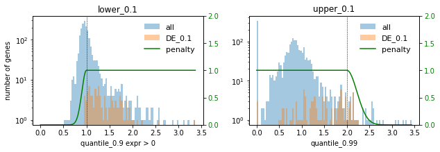
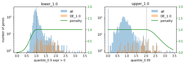
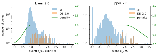
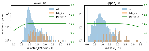
### PCA ###

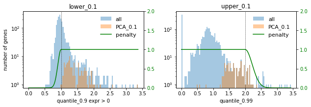
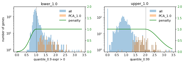
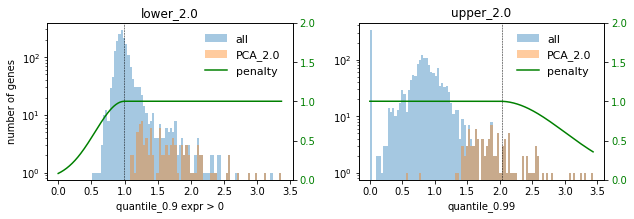
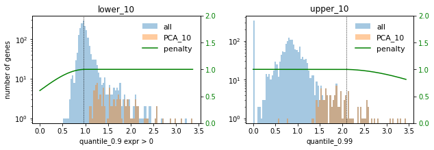
In this setting we choose the factor 0.1 to not select too many highly expressed genes. Lowly expressed genes are not selected anyway for the given selection thresholds.

We apply the expression penalties on multiple selection steps (see below). The “m_penalties<…>” would not be necessary since we don’t provide a marker list. For the case that a marker list is given the penalties should be applied as below: no lower penalty for m_penalties_list_celltypes since we don’t expect cells from that cell type expressing those markers in the given data set.

# Run selection with the calibrated expession constraints

FACTOR = 0.1

adata.var["expr_penalty_lower"] = adata.var[f"expr_penalty_lower_{FACTOR}"]
adata.var["expr_penalty_upper"] = adata.var[f"expr_penalty_upper_{FACTOR}"]

# create an instance of the ProbesetSelector class
selector = sp.se.ProbesetSelector(
    adata,
    n=None,
    celltype_key="celltype",
    verbosity=1,
    save_dir=None,
    pca_penalties=["expr_penalty_lower", "expr_penalty_upper"],
    DE_penalties=["expr_penalty_lower", "expr_penalty_upper"],
    m_penalties_adata_celltypes=["expr_penalty_lower", "expr_penalty_upper"],
    m_penalties_list_celltypes=["expr_penalty_upper"],
)


# select probe set
selector.select_probeset()

Note: The following celltypes' test set sizes for forest training are below min_test_n (=20):
         Dendritic cells : 9
         Megakaryocytes  : 3
The genes selected for those cell types potentially don't generalize well. Find the genes for each of those cell types in self.genes_of_primary_trees after running self.select_probeset().

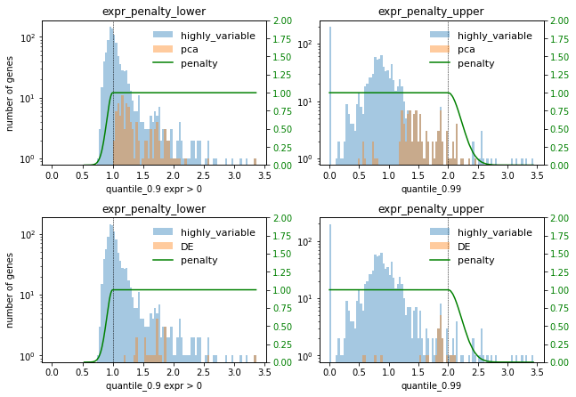
We can then investigate if the genes selected with spapros are within he expression constraints: (the selector.plot_histogram fct probably fails in spapros version 0.1.0, this will be fixed with the next release)

selector.plot_histogram(
    selections = ["pca", "DE"],
    x_axis_keys={"expr_penalty_lower": 'quantile_0.9 expr > 0', "expr_penalty_upper": 'quantile_0.99'},
    unapplied_penalty_keys={}
)

vi. Your use case is not captured?

If you face a special use case and you’re unsure if the described schemes would fit to this one, please raise an issue at our github issue section and describe the use case.

3. What’s next?

• See our basic evaluation tutorial and advanced evaluation tutorial for detailed instructions to evaluate the selected probesets.

• Check out our end to end selection tutorial for combining gene selection and probe design.