Probeset selection with Spapros

In this tutorial we showcase how to select a gene set with Spapros.

Based on a scRNA-seq reference dataset Spapros selects genes that can distinguish the cell types in that data set and capture transcriptomic varation beyond cell type labels.

In this tutorial we will use the default selection settings only. Check out the advanced selection tutorial for adjustments for specific use cases and the end-to-end probe set selection tutorial which includes the probe design.

Import packages

import scanpy as sc
import spapros as sp

sc.settings.verbosity = 0
sc.logging.print_header()
print(f"spapros=={sp.__version__}")

scanpy==1.9.1 anndata==0.8.0 umap==0.5.3 numpy==1.21.6 scipy==1.7.3 pandas==1.3.5 scikit-learn==1.0.2 statsmodels==0.13.2 python-igraph==0.9.11 pynndescent==0.5.7
spapros==0.1.0

Load and preprocess data

For Spapros selections the count data should be log-normalised. Notably genes should not be scaled to mean=0 and std=1. We pre-select a given number of highly variable genes, here 1000. In real world applications we typically go for 8000.

The example data set that we use here has a raw version and a processed version with scaled counts. To get log normalised counts we use the raw version. Cell and gene filters, cell type annotations, and the umap embedding we get from the processed version.

adata = sc.datasets.pbmc3k()
adata_tmp = sc.datasets.pbmc3k_processed()

# Get infos from the processed dataset
adata = adata[adata_tmp.obs_names,adata_tmp.var_names]
adata.obs['celltype'] = adata_tmp.obs['louvain']
adata.obsm['X_umap'] = adata_tmp.obsm['X_umap']
del adata_tmp

# Preprocess counts and get highly variable genes
sc.pp.normalize_total(adata)
sc.pp.log1p(adata)
sc.pp.highly_variable_genes(adata,flavor="cell_ranger",n_top_genes=1000)

adata

AnnData object with n_obs × n_vars = 2638 × 1838
    obs: 'celltype'
    var: 'gene_ids', 'highly_variable', 'means', 'dispersions', 'dispersions_norm'
    uns: 'log1p', 'hvg'
    obsm: 'X_umap'

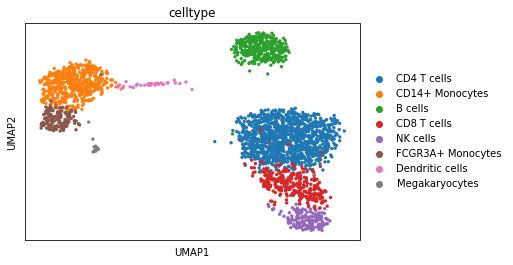
sc.pl.umap(adata,color="celltype")

Run selection

First we create an instance of the ProbesetSelector class. We specify the number of genes n (20) and the key in adata.obs where we find the cell type annotations (celltype_key="celltype"). Note that you can specify a save_dir to save results during selection and reload them next time a ProbesetSelector with the given save_dir is instantiated.

selector = sp.se.ProbesetSelector(adata, n=20, celltype_key="celltype", verbosity=1, save_dir=None)

Note: The following celltypes' test set sizes for forest training are below min_test_n (=20):
         Dendritic cells : 9
         Megakaryocytes  : 3
The genes selected for those cell types potentially don't generalize well. Find the genes for each of those cell types in self.genes_of_primary_trees after running self.select_probeset().

We get a warning that the cell type clusters for dendritic cells and megakaroycytes are quite small and therefore the genes that are selected to identify these cell types potentially don’t generalize very well. The method won’t exclude these cell types automatically, it could be done manually though by setting the parameter celltypes to a subset of cell types instead of celltypes="all".

Run the central method for probe set selection. (Takes ~5 min for the given example. Note that the progress bars should be properly displayed with jupyter notebook, however jupyter lab or e.g. vscode can lead to incomplete display)

selector.select_probeset()

The selected probeset can be examined like this:

(See the ProbesetSelector.probeset attribute for a detailed description of the output table)

selector.probeset

	gene_nr	selection	rank	marker_rank	tree_rank	importance_score	pca_score	pre_selected	prior_selected	pca_selected	celltypes_DE_1vsall	celltypes_DE_specific	celltypes_DE	celltypes_marker	list_only_ct_marker	required_marker	required_list_marker
PF4	1	True	1.0	1.0	1.0	1.000000	0.810399	False	False	True	Megakaryocytes		Megakaryocytes	Megakaryocytes	False	True	False
HLA-DPB1	2	True	1.0	1.0	1.0	0.649235	1.997253	False	False	True	B cells,Dendritic cells		B cells,Dendritic cells	B cells,Dendritic cells	False	True	False
FCGR3A	3	True	1.0	1.0	1.0	0.612390	1.321373	False	False	True		FCGR3A+ Monocytes	FCGR3A+ Monocytes	FCGR3A+ Monocytes	False	True	False
GZMB	4	True	1.0	1.0	1.0	0.512924	1.252898	False	False	True	NK cells		NK cells	NK cells	False	True	False
CCL5	5	True	1.0	1.0	1.0	0.478418	2.553322	False	False	True	CD8 T cells		CD8 T cells	CD8 T cells	False	True	False
...	...	...	...	...	...	...	...	...	...	...	...	...	...	...	...	...	...
ARHGAP19	996	False	NaN	NaN	NaN	NaN	0.016906	False	False	False					False	False	False
SLC22A4	997	False	NaN	NaN	NaN	NaN	0.016718	False	False	False					False	False	False
DRAXIN	998	False	NaN	NaN	NaN	NaN	0.016547	False	False	False					False	False	False
C1QC	999	False	NaN	NaN	NaN	NaN	0.014339	False	False	False					False	False	False
PARS2	1000	False	NaN	NaN	NaN	NaN	0.012845	False	False	False					False	False	False

1000 rows × 17 columns

The list of selected genes can be retrieved with

selector.probeset.index[selector.probeset.selection]

Index(['PF4', 'HLA-DPB1', 'FCGR3A', 'GZMB', 'CCL5', 'S100A8', 'IL32',
       'HLA-DQA1', 'NKG7', 'AIF1', 'CD79A', 'LTB', 'TYROBP', 'HLA-DMA', 'GZMK',
       'HLA-DRB1', 'FCN1', 'S100A11', 'GNLY', 'GZMH'],
      dtype='object')

Vizualize and investigate the results

Let’s first plot the mean expression in each cell type cluster with some additional information for the selected genes.

sp.pl.masked_dotplot(adata, selector)

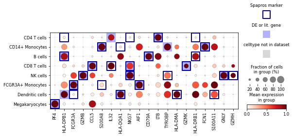
For each cell type the Spapros markers are those that build a combinatorial rule to classify the cell type. Often you find cell type specific markers, and negative markers. When selecting genes for high numbers of cell types including similar clusters the rules tend to show more sophisticated combinatorics.

The Spapros selection procedure consists of multiple steps, we can also investigate how many genes originate from the different steps:

selector.plot_gene_overlap()

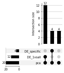
• All finally selected 20 genes occured in the PCA-based pre-selection which selects genes that capture a high amount of variation

• they strongly overlap with the (16) differentially expressed genes since marker genes are one source of high variation in transcriptomics data. The overlap is especially high for datasets with only a few cell type clusters that are also well separated as in the given example.

• The first DE tests to train optimal classification trees are tests between each cell type and all other cell types as background (DE_1vsall). To further optimise the trees we run DE tests between cell type clusters that are more difficult to distinguish (DE_specific). We find 4 genes that originate from the specific tests that didn’t occur in the 1 vs all tests.

What’s next?

You can now evaluate the selected probeset. See our basic evaluation tutorial.

If you want to customize and improve the probeset selection, have a look at the advanced selection tutorial.

Check out the end-to-end selection tutorial for the full pipline that includes probe design and gene panel selection.